En mathématiques , les intégrales trigonométriques sont une famille d'intégrales basées sur les fonctions trigonométriques .
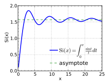
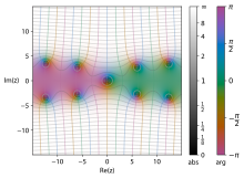
Intégrales trigonométriques Si(x ) (bleu) et Ci(x ) (vert). Sinus intégral Tracé de Si(x ) pour 0 ≤ x ≤ 8 π . Sinus intégral sur le plan complexe, tracé avec une coloration de régions . Il existe deux fonctions sinus intégrales :
Si ( x ) = ∫ 0 x sin t t d t {\displaystyle \operatorname {Si} (x)=\int _{0}^{x}{\frac {\sin t}{t}}\,\mathrm {d} t} si ( x ) = − ∫ x ∞ sin t t d t . {\displaystyle \operatorname {si} (x)=-\int _{x}^{\infty }{\frac {\sin t}{t}}\,\mathrm {d} t~.} On peut remarquer que l'intégrande sin(t )/t est la fonction sinus cardinal, et la fonction de Bessel sphérique d'ordre 0. Puisque sinc est une fonction entière paire (holomorphe sur tout le plan complexe), Si est entière, impaire, et l'intégrale dans sa définition peut être calculée le long de tout chemin reliant les extrémités.
Par définition, Si(x ) et la primitive de sin x / x qui s'annule en x = 0si(x ) est celle qui s'annule pour x → ∞intégrale de Dirichlet :
Si ( x ) − si ( x ) = ∫ 0 ∞ sin t t d t = π 2 . {\displaystyle \operatorname {Si} (x)-\operatorname {si} (x)=\int _{0}^{\infty }{\frac {\sin t}{t}}\,\mathrm {d} t={\frac {\pi }{2}}.} En traitement du signal, les oscillations du sinus intégral génèrent des suroscillations en utilisant le filtre sinus cardinal, et des suroscillations fréquentielles en utilisant un filtre sinus cardinal tronqué comme filtre passe-bas.
Ce phénomène est en lien avec le phénomène de Gibbs : si le sinus intégral est considéré comme la convolution de la fonction sinus cardinal avec la fonction de Heaviside, cela revient à tronquer la série de Fourier , d'où l'apparition du phénomène de Gibbs.
Cosinus intégral Tracé de Ci(x ) pour 0 < x ≤ 8π . Tracé de Ci(x ) sur le plan complexe entre -2-2i et 2+2i . Cosinus intégral sur le plan complexe. On peut voir la coupure le long du demi-axe des réels négatifs. Il existe deux fonctions cosinus intégrales :
Ci ( x ) = − ∫ x ∞ cos t t d t {\displaystyle \operatorname {Ci} (x)=-\int _{x}^{\infty }{\frac {\cos t}{t}}\,\mathrm {d} t} Cin ( x ) = ∫ 0 x 1 − cos t t d t = γ + ln x − Ci ( x ) pour | Arg ( x ) | < π , {\displaystyle \operatorname {Cin} (x)=\int _{0}^{x}{\frac {1-\cos t}{t}}\,\mathrm {d} t=\gamma +\ln x-\operatorname {Ci} (x)\qquad ~{\text{ pour }}~\left|\operatorname {Arg} (x)\right|<\pi ~,} où γ ≈ 0.57721566 ...constante d'Euler-Mascheroni . Certains textes utilisent la notation ci au lieu de Ci .
Ci(x ) est la primitive de cos(x )/x qui s'annule pour x → ∞
Cin est une fonction entière paire . Pour cela, certains auteurs préfèrent définir Cin puis en déduire Ci .
Généralisations Les fonctions intégrales généralisées sont définies, pour x réel positif, par[ 1]
∀ z ∈ C , 0 < ℜ ( z ) < 2 , S i ( x , z ) = ∫ 0 x sin ( t ) t z d t , {\displaystyle \forall z\in \mathbb {C} ,\ 0<\Re (z)<2,\ \mathrm {Si} (x,z)=\int _{0}^{x}{\frac {\sin(t)}{t^{z}}}~\mathrm {d} t,} ∀ z ∈ C , 0 < ℜ ( z ) < 1 , C i ( x , z ) = ∫ 0 x cos ( t ) t z d t {\displaystyle \forall z\in \mathbb {C} ,\ 0<\Re (z)<1,\ \mathrm {Ci} (x,z)=\int _{0}^{x}{\frac {\cos(t)}{t^{z}}}~\mathrm {d} t} On a alors :
S i ( x , 0 ) = 1 − cos ( x ) , C i ( x , 0 ) = sin ( x ) {\displaystyle \mathrm {Si} (x,0)=1-\cos(x),\ \mathrm {Ci} (x,0)=\sin(x)} S i ( x , 1 ) = S i ( x ) , C i ( x , 1 ) = ∫ 0 + i n f t y cos ( t ) t z d t − C i ( x ) {\displaystyle \mathrm {Si} (x,1)=\mathrm {Si} (x),\ \mathrm {Ci} (x,1)=\int _{0}^{+infty}{\frac {\cos(t)}{t^{z}}}~\mathrm {d} t-\mathrm {Ci} (x)} S i ( x , 1 / 2 ) = 2 S ( x ) , C i ( x , 1 / 2 ) = 2 C ( x ) {\displaystyle \mathrm {Si} (x,1/2)=2S({\sqrt {x}}),\,\mathrm {Ci} (x,1/2)=2C({\sqrt {x}})} S et C sont les fonctions de Fresnel .Ces fonctions ont été utilisées dans l'étude du phénomène de Gibbs .
Intégrales trigonométriques hyperboliques Sinus hyperbolique intégral Tracé de Shi(x ) sur le plan complexe entre -2-2i et 2+2i . Le sinus hyperbolique intégral est défini par
Shi ( x ) = ∫ 0 x sinh ( t ) t d t . {\displaystyle \operatorname {Shi} (x)=\int _{0}^{x}{\frac {\sinh(t)}{t}}\,\mathrm {d} t.} On peut la relier à la fonction sinus intégral par l'égalité :
Si ( i x ) = i Shi ( x ) . {\displaystyle \operatorname {Si} (\mathrm {i} x)=\mathrm {i} \operatorname {Shi} (x).}
Cosinus hyperbolique intégral Tracé de Chi(x ) sur le plan complexe entre -2-2i et 2+2i . Le cosinus hyperbolique intégral est défini par
Chi ( x ) = γ + ln x + ∫ 0 x cosh t − 1 t d t pour | Arg ( x ) | < π , {\displaystyle \operatorname {Chi} (x)=\gamma +\ln x+\int _{0}^{x}{\frac {\cosh t-1}{t}}\,\mathrm {d} t\qquad ~{\text{ pour }}~\left|\operatorname {Arg} (x)\right|<\pi ~,} où
γ {\displaystyle \gamma } est la
constante d'Euler-Mascheroni .
Il a pour développement limité
Chi ( x ) = γ + ln ( x ) + x 2 4 + x 4 96 + x 6 4320 + x 8 322560 + x 10 36288000 + O ( x 12 ) . {\displaystyle \operatorname {Chi} (x)=\gamma +\ln(x)+{\frac {x^{2}}{4}}+{\frac {x^{4}}{96}}+{\frac {x^{6}}{4320}}+{\frac {x^{8}}{322560}}+{\frac {x^{10}}{36288000}}+O(x^{12}).}
Fonctions auxiliaires Les intégrales trigonométriques peuvent être vues en termes de "fonctions auxiliaires"
f ( x ) ≡ ∫ 0 ∞ sin ( t ) t + x d t = ∫ 0 ∞ e − x t t 2 + 1 d t = Ci ( x ) sin ( x ) + [ π 2 − Si ( x ) ] cos ( x ) , g ( x ) ≡ ∫ 0 ∞ cos ( t ) t + x d t = ∫ 0 ∞ t e − x t t 2 + 1 d t = − Ci ( x ) cos ( x ) + [ π 2 − Si ( x ) ] sin ( x ) . {\displaystyle {\begin{aligned}f(x)\equiv &\int _{0}^{\infty }{\frac {\sin(t)}{t+x}}\,\mathrm {d} t&=&\int _{0}^{\infty }{\frac {\mathrm {e} ^{-xt}}{t^{2}+1}}\,\mathrm {d} t&=&\operatorname {Ci} (x)\sin(x)+\left[{\frac {\pi }{2}}-\operatorname {Si} (x)\right]\cos(x)~,\\[5pt]g(x)\equiv &\int _{0}^{\infty }{\frac {\cos(t)}{t+x}}\,\mathrm {d} t&=&\int _{0}^{\infty }{\frac {t\mathrm {e} ^{-xt}}{t^{2}+1}}\,\mathrm {d} t&=&-\operatorname {Ci} (x)\cos(x)+\left[{\frac {\pi }{2}}-\operatorname {Si} (x)\right]\sin(x)~.\end{aligned}}} A partir de ces fonctions, les intégrales trigonométriques peuvent être réécrites en (cf. Abramowitz & Stegun, p. 232)
π 2 − Si ( x ) = − si ( x ) = f ( x ) cos ( x ) + g ( x ) sin ( x ) , et Ci ( x ) = f ( x ) sin ( x ) − g ( x ) cos ( x ) . {\displaystyle {\begin{array}{rcl}{\frac {\pi }{2}}-\operatorname {Si} (x)=-\operatorname {si} (x)&=&f(x)\cos(x)+g(x)\sin(x)~,\qquad {\text{ et }}\\\operatorname {Ci} (x)&=&f(x)\sin(x)-g(x)\cos(x)~.\\\end{array}}} Spirale de Nielsen Spirale de Nielsen. La spirale paramétrée par les fonctions si , ci est connue comme la spirale de Nielsen :
{ x ( t ) = a × ci ( t ) y ( t ) = a × si ( t ) {\displaystyle {\begin{cases}x(t)=a\times \operatorname {ci} (t)\\y(t)=a\times \operatorname {si} (t)\end{cases}}} La spirale est liée aux intégrales de Fresnel et la spirale d'Euler . La spirale de Nielsen a des applications en traitement de la vision, constructions de route, entre autres[ 2]
Développements Selon la valeur de l'argument, on pourra choisir différentes écritures de développements des intégrales trigonométriques.
Séries asymptotiques
Si ( x ) ∼ π 2 − cos x x ( 1 − 2 ! x 2 + 4 ! x 4 − 6 ! x 6 ⋯ ) − sin x x ( 1 x − 3 ! x 3 + 5 ! x 5 − 7 ! x 7 ⋯ ) {\displaystyle \operatorname {Si} (x)\sim {\frac {\pi }{2}}-{\frac {\cos x}{x}}\left(1-{\frac {2!}{x^{2}}}+{\frac {4!}{x^{4}}}-{\frac {6!}{x^{6}}}\cdots \right)-{\frac {\sin x}{x}}\left({\frac {1}{x}}-{\frac {3!}{x^{3}}}+{\frac {5!}{x^{5}}}-{\frac {7!}{x^{7}}}\cdots \right)} Ci ( x ) ∼ sin x x ( 1 − 2 ! x 2 + 4 ! x 4 − 6 ! x 6 ⋯ ) − cos x x ( 1 x − 3 ! x 3 + 5 ! x 5 − 7 ! x 7 ⋯ ) . {\displaystyle \operatorname {Ci} (x)\sim {\frac {\sin x}{x}}\left(1-{\frac {2!}{x^{2}}}+{\frac {4!}{x^{4}}}-{\frac {6!}{x^{6}}}\cdots \right)-{\frac {\cos x}{x}}\left({\frac {1}{x}}-{\frac {3!}{x^{3}}}+{\frac {5!}{x^{5}}}-{\frac {7!}{x^{7}}}\cdots \right)~.} Ces séries sont asymptotiques et divergentes, mais peuvent être utilisées pour des estimations et évaluations dès que ℜ(x ) ≫ 1 .
Séries convergentes Les développements suivants se déduisent des séries de Maclaurin du sinus et du cosinus :
Si ( x ) = ∑ n = 0 ∞ ( − 1 ) n x 2 n + 1 ( 2 n + 1 ) ( 2 n + 1 ) ! = x − x 3 3 ! ⋅ 3 + x 5 5 ! ⋅ 5 − x 7 7 ! ⋅ 7 ± ⋯ {\displaystyle \operatorname {Si} (x)=\sum _{n=0}^{\infty }{\frac {(-1)^{n}x^{2n+1}}{(2n+1)(2n+1)!}}=x-{\frac {x^{3}}{3!\cdot 3}}+{\frac {x^{5}}{5!\cdot 5}}-{\frac {x^{7}}{7!\cdot 7}}\pm \cdots } Ci ( x ) = γ + ln x + ∑ n = 1 ∞ ( − 1 ) n x 2 n 2 n ( 2 n ) ! = γ + ln x − x 2 2 ! ⋅ 2 + x 4 4 ! ⋅ 4 ∓ ⋯ {\displaystyle \operatorname {Ci} (x)=\gamma +\ln x+\sum _{n=1}^{\infty }{\frac {(-1)^{n}x^{2n}}{2n(2n)!}}=\gamma +\ln x-{\frac {x^{2}}{2!\cdot 2}}+{\frac {x^{4}}{4!\cdot 4}}\mp \cdots } Elles sont convergentes pour tout complexe x , mais pour |x , la convergence lente va imposer d'utiliser un grand nombre de termes.
Relation avec l'exponentielle intégrale d'argument imaginaire On considère la fonction exponentielle intégrale
E 1 ( z ) = ∫ 1 ∞ exp ( − z t ) t d t pour ℜ ( z ) ≥ 0. {\displaystyle \operatorname {E} _{1}(z)=\int _{1}^{\infty }{\frac {\exp(-zt)}{t}}\,\mathrm {d} t\qquad ~{\text{ pour }}~\Re (z)\geq 0.} Elle est très proche des fonctions
Si et
Ci :
E 1 ( i x ) = i ( − π 2 + Si ( x ) ) − Ci ( x ) = i si ( x ) − ci ( x ) pour x > 0 . {\displaystyle \operatorname {E} _{1}(\mathrm {i} x)=\mathrm {i} \left(-{\frac {\pi }{2}}+\operatorname {Si} (x)\right)-\operatorname {Ci} (x)=\mathrm {i} \operatorname {si} (x)-\operatorname {ci} (x)\qquad ~{\text{ pour }}~x>0~.} Comme toutes ces fonctions sont analytiques sauf sur la branche des valeurs négatives de l'argument, le domaine de validité de la relation doit être étendu à (hors de ce domaine, des termes additionnels sous forme de facteurs entiers de π apparaissent.)
Les cas de l'argument imaginaire pur de la fonction exponentielle intégrale sont
∫ 1 ∞ cos ( a x ) ln x x d x = − π 2 24 + γ ( γ 2 + ln a ) + ln 2 a 2 + ∑ n ≥ 1 ( − a 2 ) n ( 2 n ) ! ( 2 n ) 2 , {\displaystyle \int _{1}^{\infty }\cos(ax){\frac {\ln x}{x}}\,\mathrm {d} x=-{\frac {\pi ^{2}}{24}}+\gamma \left({\frac {\gamma }{2}}+\ln a\right)+{\frac {\ln ^{2}a}{2}}+\sum _{n\geq 1}{\frac {(-a^{2})^{n}}{(2n)!\,(2n)^{2}}}~,} qui est la partie réelle de
∫ 1 ∞ e i a x ln x x d x = − π 2 24 + γ ( γ 2 + ln a ) + ln 2 a 2 − π 2 i ( γ + ln a ) + ∑ n ≥ 1 ( i a ) n n ! n 2 . {\displaystyle \int _{1}^{\infty }\mathrm {e} ^{\mathrm {i} ax}{\frac {\ln x}{x}}\,\mathrm {d} x=-{\frac {\pi ^{2}}{24}}+\gamma \left({\frac {\gamma }{2}}+\ln a\right)+{\frac {\ln ^{2}a}{2}}-{\frac {\pi }{2}}\mathrm {i} \left(\gamma +\ln a\right)+\sum _{n\geq 1}{\frac {(\mathrm {i} a)^{n}}{n!\,n^{2}}}~.} De façon similaire,
∫ 1 ∞ e i a x ln x x 2 d x = 1 + i a [ − π 2 24 + γ ( γ 2 + ln a − 1 ) + ln 2 a 2 − ln a + 1 ] + π a 2 ( γ + ln a − 1 ) + ∑ n ≥ 1 ( i a ) n + 1 ( n + 1 ) ! n 2 . {\displaystyle \int _{1}^{\infty }\mathrm {e} ^{\mathrm {i} ax}{\frac {\ln x}{x^{2}}}\,\mathrm {d} x=1+\mathrm {i} a\left[-{\frac {\pi ^{2}}{24}}+\gamma \left({\frac {\gamma }{2}}+\ln a-1\right)+{\frac {\ln ^{2}a}{2}}-\ln a+1\right]+{\frac {\pi a}{2}}\left(\gamma +\ln a-1\right)+\sum _{n\geq 1}{\frac {(\mathrm {i} a)^{n+1}}{(n+1)!\,n^{2}}}~.} Méthodes de calcul efficaces Les approximants de Padé des séries de Taylor convergentes donnent une méthode efficace d'évaluation des fonctions pour de petits arguments. Les formules suivantes, données par Rowe et al. (2015)[ 3] 10−16 pour 0 ≤ x ≤ 4 ,
Si ( x ) ≈ x ⋅ ( 1 − 4 , 54393409816329991 ⋅ 10 − 2 ⋅ x 2 + 1 , 15457225751016682 ⋅ 10 − 3 ⋅ x 4 − 1 , 41018536821330254 ⋅ 10 − 5 ⋅ x 6 + 9 , 43280809438713025 ⋅ 10 − 8 ⋅ x 8 − 3 , 53201978997168357 ⋅ 10 − 10 ⋅ x 10 + 7 , 08240282274875911 ⋅ 10 − 13 ⋅ x 12 − 6 , 05338212010422477 ⋅ 10 − 16 ⋅ x 14 1 + 1 , 01162145739225565 ⋅ 10 − 2 ⋅ x 2 + 4 , 99175116169755106 ⋅ 10 − 5 ⋅ x 4 + 1 , 55654986308745614 ⋅ 10 − 7 ⋅ x 6 + 3 , 28067571055789734 ⋅ 10 − 10 ⋅ x 8 + 4 , 5049097575386581 ⋅ 10 − 13 ⋅ x 10 + 3 , 21107051193712168 ⋅ 10 − 16 ⋅ x 12 ) Ci ( x ) ≈ γ + ln ( x ) + x 2 ⋅ ( − 0 , 25 + 7 , 51851524438898291 ⋅ 10 − 3 ⋅ x 2 − 1 , 27528342240267686 ⋅ 10 − 4 ⋅ x 4 + 1 , 05297363846239184 ⋅ 10 − 6 ⋅ x 6 − 4 , 68889508144848019 ⋅ 10 − 9 ⋅ x 8 + 1 , 06480802891189243 ⋅ 10 − 11 ⋅ x 10 − 9 , 93728488857585407 ⋅ 10 − 15 ⋅ x 12 1 + 1 , 1592605689110735 ⋅ 10 − 2 ⋅ x 2 + 6 , 72126800814254432 ⋅ 10 − 5 ⋅ x 4 + 2 , 55533277086129636 ⋅ 10 − 7 ⋅ x 6 + 6 , 97071295760958946 ⋅ 10 − 10 ⋅ x 8 + 1 , 38536352772778619 ⋅ 10 − 12 ⋅ x 10 + 1 , 89106054713059759 ⋅ 10 − 15 ⋅ x 12 + 1 , 39759616731376855 ⋅ 10 − 18 ⋅ x 14 ) {\displaystyle {\begin{array}{rcl}\operatorname {Si} (x)&\approx &x\cdot \left({\frac {\begin{array}{l}1-4,54393409816329991\cdot 10^{-2}\cdot x^{2}+1,15457225751016682\cdot 10^{-3}\cdot x^{4}-1,41018536821330254\cdot 10^{-5}\cdot x^{6}\\~~~+9,43280809438713025\cdot 10^{-8}\cdot x^{8}-3,53201978997168357\cdot 10^{-10}\cdot x^{10}+7,08240282274875911\cdot 10^{-13}\cdot x^{12}\\~~~-6,05338212010422477\cdot 10^{-16}\cdot x^{14}\end{array}}{\begin{array}{l}1+1,01162145739225565\cdot 10^{-2}\cdot x^{2}+4,99175116169755106\cdot 10^{-5}\cdot x^{4}+1,55654986308745614\cdot 10^{-7}\cdot x^{6}\\~~~+3,28067571055789734\cdot 10^{-10}\cdot x^{8}+4,5049097575386581\cdot 10^{-13}\cdot x^{10}+3,21107051193712168\cdot 10^{-16}\cdot x^{12}\end{array}}}\right)\\&~&\\\operatorname {Ci} (x)&\approx &\gamma +\ln(x)+x^{2}\cdot \left({\frac {\begin{array}{l}-0,25+7,51851524438898291\cdot 10^{-3}\cdot x^{2}-1,27528342240267686\cdot 10^{-4}\cdot x^{4}+1,05297363846239184\cdot 10^{-6}\cdot x^{6}\\~~~-4,68889508144848019\cdot 10^{-9}\cdot x^{8}+1,06480802891189243\cdot 10^{-11}\cdot x^{10}-9,93728488857585407\cdot 10^{-15}\cdot x^{12}\\\end{array}}{\begin{array}{l}1+1,1592605689110735\cdot 10^{-2}\cdot x^{2}+6,72126800814254432\cdot 10^{-5}\cdot x^{4}+2,55533277086129636\cdot 10^{-7}\cdot x^{6}\\~~~+6,97071295760958946\cdot 10^{-10}\cdot x^{8}+1,38536352772778619\cdot 10^{-12}\cdot x^{10}+1,89106054713059759\cdot 10^{-15}\cdot x^{12}\\~~~+1,39759616731376855\cdot 10^{-18}\cdot x^{14}\\\end{array}}}\right)\end{array}}} Les intégrales peuvent également être évaluées indirectement par les fonctions auxiliaires f ( x ) {\displaystyle f(x)} g ( x ) {\displaystyle g(x)}
Pour x ≥ 4, les fonctions rationnelles de Padé ci-dessous approchent f ( x ) {\displaystyle f(x)} g ( x ) {\displaystyle g(x)} 10−16 [ 3]
f ( x ) ≈ 1 x ⋅ ( 1 + 7 , 44437068161936700618 ⋅ 10 2 ⋅ x − 2 + 1 , 96396372895146869801 ⋅ 10 5 ⋅ x − 4 + 2 , 37750310125431834034 ⋅ 10 7 ⋅ x − 6 + 1 , 43073403821274636888 ⋅ 10 9 ⋅ x − 8 + 4 , 33736238870432522765 ⋅ 10 10 ⋅ x − 10 + 6 , 40533830574022022911 ⋅ 10 11 ⋅ x − 12 + 4 , 20968180571076940208 ⋅ 10 12 ⋅ x − 14 + 1 , 00795182980368574617 ⋅ 10 13 ⋅ x − 16 + 4 , 94816688199951963482 ⋅ 10 12 ⋅ x − 18 − 4 , 94701168645415959931 ⋅ 10 11 ⋅ x − 20 1 + 7 , 46437068161927678031 ⋅ 10 2 ⋅ x − 2 + 1 , 97865247031583951450 ⋅ 10 5 ⋅ x − 4 + 2 , 41535670165126845144 ⋅ 10 7 ⋅ x − 6 + 1 , 47478952192985464958 ⋅ 10 9 ⋅ x − 8 + 4 , 58595115847765779830 ⋅ 10 10 ⋅ x − 10 + 7 , 08501308149515401563 ⋅ 10 11 ⋅ x − 12 + 5 , 06084464593475076774 ⋅ 10 12 ⋅ x − 14 + 1 , 43468549171581016479 ⋅ 10 13 ⋅ x − 16 + 1 , 11535493509914254097 ⋅ 10 13 ⋅ x − 18 ) g ( x ) ≈ 1 x 2 ⋅ ( 1 + 8 , 1359520115168615 ⋅ 10 2 ⋅ x − 2 + 2 , 35239181626478200 ⋅ 10 5 ⋅ x − 4 + 3 , 12557570795778731 ⋅ 10 7 ⋅ x − 6 + 2 , 06297595146763354 ⋅ 10 9 ⋅ x − 8 + 6 , 83052205423625007 ⋅ 10 10 ⋅ x − 10 + 1 , 09049528450362786 ⋅ 10 12 ⋅ x − 12 + 7 , 57664583257834349 ⋅ 10 12 ⋅ x − 14 + 1 , 81004487464664575 ⋅ 10 13 ⋅ x − 16 + 6 , 43291613143049485 ⋅ 10 12 ⋅ x − 18 − 1 , 36517137670871689 ⋅ 10 12 ⋅ x − 20 1 + 8 , 19595201151451564 ⋅ 10 2 ⋅ x − 2 + 2 , 40036752835578777 ⋅ 10 5 ⋅ x − 4 + 3 , 26026661647090822 ⋅ 10 7 ⋅ x − 6 + 2 , 23355543278099360 ⋅ 10 9 ⋅ x − 8 + 7 , 87465017341829930 ⋅ 10 10 ⋅ x − 10 + 1 , 39866710696414565 ⋅ 10 12 ⋅ x − 12 + 1 , 7164723371736605 ⋅ 10 13 ⋅ x − 14 + 4 , 01839087307656620 ⋅ 10 13 ⋅ x − 16 + 3 , 99653257887490811 ⋅ 10 13 ⋅ x − 18 ) {\displaystyle {\begin{array}{rcl}f(x)&\approx &{\dfrac {1}{x}}\cdot \left({\frac {\begin{array}{l}1+7,44437068161936700618\cdot 10^{2}\cdot x^{-2}+1,96396372895146869801\cdot 10^{5}\cdot x^{-4}+2,37750310125431834034\cdot 10^{7}\cdot x^{-6}\\~~~+1,43073403821274636888\cdot 10^{9}\cdot x^{-8}+4,33736238870432522765\cdot 10^{10}\cdot x^{-10}+6,40533830574022022911\cdot 10^{11}\cdot x^{-12}\\~~~+4,20968180571076940208\cdot 10^{12}\cdot x^{-14}+1,00795182980368574617\cdot 10^{13}\cdot x^{-16}+4,94816688199951963482\cdot 10^{12}\cdot x^{-18}\\~~~-4,94701168645415959931\cdot 10^{11}\cdot x^{-20}\end{array}}{\begin{array}{l}1+7,46437068161927678031\cdot 10^{2}\cdot x^{-2}+1,97865247031583951450\cdot 10^{5}\cdot x^{-4}+2,41535670165126845144\cdot 10^{7}\cdot x^{-6}\\~~~+1,47478952192985464958\cdot 10^{9}\cdot x^{-8}+4,58595115847765779830\cdot 10^{10}\cdot x^{-10}+7,08501308149515401563\cdot 10^{11}\cdot x^{-12}\\~~~+5,06084464593475076774\cdot 10^{12}\cdot x^{-14}+1,43468549171581016479\cdot 10^{13}\cdot x^{-16}+1,11535493509914254097\cdot 10^{13}\cdot x^{-18}\end{array}}}\right)\\&&\\g(x)&\approx &{\dfrac {1}{x^{2}}}\cdot \left({\frac {\begin{array}{l}1+8,1359520115168615\cdot 10^{2}\cdot x^{-2}+2,35239181626478200\cdot 10^{5}\cdot x^{-4}+3,12557570795778731\cdot 10^{7}\cdot x^{-6}\\~~~+2,06297595146763354\cdot 10^{9}\cdot x^{-8}+6,83052205423625007\cdot 10^{10}\cdot x^{-10}+1,09049528450362786\cdot 10^{12}\cdot x^{-12}\\~~~+7,57664583257834349\cdot 10^{12}\cdot x^{-14}+1,81004487464664575\cdot 10^{13}\cdot x^{-16}+6,43291613143049485\cdot 10^{12}\cdot x^{-18}\\~~~-1,36517137670871689\cdot 10^{12}\cdot x^{-20}\end{array}}{\begin{array}{l}1+8,19595201151451564\cdot 10^{2}\cdot x^{-2}+2,40036752835578777\cdot 10^{5}\cdot x^{-4}+3,26026661647090822\cdot 10^{7}\cdot x^{-6}\\~~~+2,23355543278099360\cdot 10^{9}\cdot x^{-8}+7,87465017341829930\cdot 10^{10}\cdot x^{-10}+1,39866710696414565\cdot 10^{12}\cdot x^{-12}\\~~~+1,7164723371736605\cdot 10^{13}\cdot x^{-14}+4,01839087307656620\cdot 10^{13}\cdot x^{-16}+3,99653257887490811\cdot 10^{13}\cdot x^{-18}\end{array}}}\right)\\\end{array}}} Voir aussi Références (en) Cet article est partiellement ou en totalité issu de l’article de Wikipédia en anglais intitulé « Trigonometric integral » (voir la liste des auteurs) . ↑ (de) E. Kreyszig, « Über den allgemeinen Integralsinus Si(z , a ) », Acta Mathematica vol. 85, 1951 , p. 117-181 (DOI 10.1007/BF02395744 ) ↑ Gray , Modern Differential Geometry of Curves and Surfaces. , Boca Raton, 1993 , 119 p. ↑ a et b B. Rowe et al. GALSIM: The modular galaxy image simulation toolkit », Astronomy and Computing , vol. 10, 2015 , p. 121 (DOI 10.1016/j.ascom.2015.02.002 , Bibcode 2015A&C....10..121R , arXiv 1407.7676 , S2CID 62709903 ) Bibliographie (en) Richard J. Mathar, « Numerical evaluation of the oscillatory integral over exp(iπx )·x 1/x between 1 and ∞ », 2009 .Appendix B W.H. Press , S.A. Teukolsky , W.T. Vetterling et B.P. Flannery , Numerical Recipes: The Art of Scientific Computing , New York, Cambridge University Press, 2007 , 3rd éd. (ISBN 978-0-521-88068-8 , lire en ligne) , « Section 6.8.2 – Cosine and Sine Integrals » (en) Mircea E. Șelariu, Florentin Smarandache et Marian Nițu, « Cardinal Functions and Integral Functions », International Journal of Geometry vol. 1, no 1, 2012 , p. 27-40 (lire en ligne) (en) (en) N.M. Temme , « Exponential, Logarithmic, Sine, and Cosine Integrals », sur NIST Handbook of Mathematical Functions 2010 (ISBN 978-0521192255 ) Liens externes (en) Eric W. Weisstein , « Sine Integral MathWorld (en) « Integral sine » , dans Michiel Hazewinkel , Encyclopædia of Mathematics Springer , 2002 (ISBN 978-1556080104 , lire en ligne) (en) « Integral cosine » , dans Michiel Hazewinkel , Encyclopædia of Mathematics Springer , 2002 (ISBN 978-1556080104 , lire en ligne) Portail de l'analyse 


![{\displaystyle {\begin{aligned}f(x)\equiv &\int _{0}^{\infty }{\frac {\sin(t)}{t+x}}\,\mathrm {d} t&=&\int _{0}^{\infty }{\frac {\mathrm {e} ^{-xt}}{t^{2}+1}}\,\mathrm {d} t&=&\operatorname {Ci} (x)\sin(x)+\left[{\frac {\pi }{2}}-\operatorname {Si} (x)\right]\cos(x)~,\\[5pt]g(x)\equiv &\int _{0}^{\infty }{\frac {\cos(t)}{t+x}}\,\mathrm {d} t&=&\int _{0}^{\infty }{\frac {t\mathrm {e} ^{-xt}}{t^{2}+1}}\,\mathrm {d} t&=&-\operatorname {Ci} (x)\cos(x)+\left[{\frac {\pi }{2}}-\operatorname {Si} (x)\right]\sin(x)~.\end{aligned}}}](https://wikimedia.org/api/rest_v1/media/math/render/svg/ea60947c6d639f2550728c1feb5a58ff360692dc)


![{\displaystyle \int _{1}^{\infty }\mathrm {e} ^{\mathrm {i} ax}{\frac {\ln x}{x^{2}}}\,\mathrm {d} x=1+\mathrm {i} a\left[-{\frac {\pi ^{2}}{24}}+\gamma \left({\frac {\gamma }{2}}+\ln a-1\right)+{\frac {\ln ^{2}a}{2}}-\ln a+1\right]+{\frac {\pi a}{2}}\left(\gamma +\ln a-1\right)+\sum _{n\geq 1}{\frac {(\mathrm {i} a)^{n+1}}{(n+1)!\,n^{2}}}~.}](https://wikimedia.org/api/rest_v1/media/math/render/svg/fad479e819d78322c9ce8f675cfc25a7e2f35667)


 Portail de l'analyse


