Fonction de test pour l'optimisation
En mathématiques appliquées, les fonctions de test sont des fonctions d'évaluation des caractéristiques des algorithmes d'optimisation, telles que taux de convergence ; précision ; robustesse ; performances générales.
Cette page représente que les fonctions de test les plus classiques:
- à objectif unique.
- multi-objectifs (MOP), avec leur fronts de Pareto.
Les représentations graphiques sont tirés de Bäck[1], Haupt et al.[2] et du logiciel Rody Oldenhuis[3]. Compte tenu du nombre de problèmes (55 au total), seuls quelques-uns sont présentés ici.
Les fonctions de test utilisées pour évaluer les algorithmes de MOP sont tirées de Deb[4], Binh et al.[5] et Binh[6]. On peut télécharger le logiciel développé par Deb[7], qui implémente la procédure NSGA-II avec GAs, ou le programme mis en ligne sur Internet[8], qui implémente la procédure NSGA-II avec ES.
Dans les présentations suivantes, seront juste données la forme générale de l'équation, un tracé de la fonction objectif, les limites des variables d'objet et les coordonnées des minima globaux.
Optimisations à objectif unique
| Nom | Représentation | Formule | Minimum absolu | Domaine d'application |
|---|---|---|---|---|
| Rastrigin function | 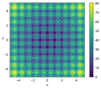 |
| ||
| Fonction d'Ackley | 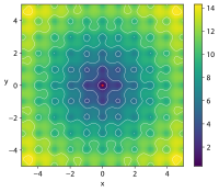 |
| ||
| Sphère |  | , | ||
| Rosenbrock function |  | , | ||
| Fonction de Beale |  |
| ||
| Goldstein–Price |  |
| ||
| Booth |  | |||
| Bukin N.6 |  | , | ||
| Fonction de Matyas |  | |||
| Fonction de Lévi N.13 |  |
| ||
| Himmelblau's function |  | |||
| Three-hump camel |  | |||
| Easom |  | |||
| Cross-in-tray |  | |||
| Eggholder[9] | 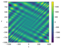 | |||
| Table de Hölder |  | |||
| McCormick |  | , | ||
| Schaffer N. 2 |  | |||
| Schaffer N. 4 |  | |||
| Styblinski–Tang |  | , .. |
![{\displaystyle f(\mathbf {x} )=An+\sum _{i=1}^{n}\left[x_{i}^{2}-A\cos(2\pi x_{i})\right]}](https://wikimedia.org/api/rest_v1/media/math/render/svg/1aa1c38ee739ca9cf4582867d74d469df4676cbc)


![{\displaystyle f(x,y)=-20\exp \left[-0.2{\sqrt {0.5\left(x^{2}+y^{2}\right)}}\right]}](https://wikimedia.org/api/rest_v1/media/math/render/svg/7f00d1325d65d088f8ae6a96137e62021107921d)
![{\displaystyle -\exp \left[0.5\left(\cos 2\pi x+\cos 2\pi y\right)\right]+e+20}](https://wikimedia.org/api/rest_v1/media/math/render/svg/565ef43958a50fb0ef473bdd46e30bfc725604a7)


![{\displaystyle f({\boldsymbol {x}})=\sum _{i=1}^{n-1}\left[100\left(x_{i+1}-x_{i}^{2}\right)^{2}+\left(1-x_{i}\right)^{2}\right]}](https://wikimedia.org/api/rest_v1/media/math/render/svg/64863353dcdea2f0ed049cec3aea0a4284d4916a)


![{\displaystyle f(x,y)=\left[1+\left(x+y+1\right)^{2}\left(19-14x+3x^{2}-14y+6xy+3y^{2}\right)\right]}](https://wikimedia.org/api/rest_v1/media/math/render/svg/2d020ed324ff07759faf17591157771b0e2cdf07)
![{\displaystyle \left[30+\left(2x-3y\right)^{2}\left(18-32x+12x^{2}+48y-36xy+27y^{2}\right)\right]}](https://wikimedia.org/api/rest_v1/media/math/render/svg/32e562da4f3219f9d66e059441c59e1d299e8557)


![{\displaystyle f(x,y)=-0.0001\left[\left|\sin x\sin y\exp \left(\left|100-{\frac {\sqrt {x^{2}+y^{2}}}{\pi }}\right|\right)\right|+1\right]^{0.1}}](https://wikimedia.org/api/rest_v1/media/math/render/svg/d591ae9bcf2feae162cd00398d78bb6870c82946)


![{\displaystyle f(x,y)=0.5+{\frac {\sin ^{2}\left(x^{2}-y^{2}\right)-0.5}{\left[1+0.001\left(x^{2}+y^{2}\right)\right]^{2}}}}](https://wikimedia.org/api/rest_v1/media/math/render/svg/995008c6f10a14b44dac568cc544efb7d5ddd631)
![{\displaystyle f(x,y)=0.5+{\frac {\cos ^{2}\left[\sin \left(\left|x^{2}-y^{2}\right|\right)\right]-0.5}{\left[1+0.001\left(x^{2}+y^{2}\right)\right]^{2}}}}](https://wikimedia.org/api/rest_v1/media/math/render/svg/2458c352c0c0524648d8ef713bcea4e80df32fd8)


Optimisations contraintes
| Name | Plot | Formula | Global minimum | Search domain |
|---|---|---|---|---|
| Rosenbrock function constrained with a cubic and a line[10] |  | , subjected to: | , | |
| Rosenbrock function constrained to a disk[11] |  | , subjected to: | , | |
| Mishra's Bird function - constrained[12],[13] |  | , subjected to: | , | |
| Townsend function (modified)[14] |  | , subjected to: where: t = Atan2(x,y) | , | |
| Gomez and Levy function (modified)[15] |  | , subjected to: | , | |
| Simionescu function[16] |  | , subjected to: |


![{\displaystyle f(x,y)=\sin(y)e^{\left[(1-\cos x)^{2}\right]}+\cos(x)e^{\left[(1-\sin y)^{2}\right]}+(x-y)^{2}}](https://wikimedia.org/api/rest_v1/media/math/render/svg/7987d4a794d861e7ccd0795265841d3ca172cfae)


![{\displaystyle f(x,y)=-[\cos((x-0.1)y)]^{2}-x\sin(3x+y)}](https://wikimedia.org/api/rest_v1/media/math/render/svg/8dac25f97d0b720512d72c313000d5fb5c7d033a)
![{\displaystyle x^{2}+y^{2}<\left[2\cos t-{\frac {1}{2}}\cos 2t-{\frac {1}{4}}\cos 3t-{\frac {1}{8}}\cos 4t\right]^{2}+[2\sin t]^{2}}](https://wikimedia.org/api/rest_v1/media/math/render/svg/57168b192e685c6144e3a9527b12087ac7cb11b4)


![{\displaystyle x^{2}+y^{2}\leq \left[r_{T}+r_{S}\cos \left(n\arctan {\frac {x}{y}}\right)\right]^{2}}](https://wikimedia.org/api/rest_v1/media/math/render/svg/1fc42adcc2095ed0c0214a74799db7ee2fac9923)


Optimisations multi-objectifs
| Name | Plot | Functions | Constraints | Search domain |
|---|---|---|---|---|
| Binh and Korn function: | 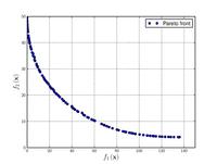 | , | ||
| Chankong and Haimes function[17] : |  | |||
| Fonseca–Fleming function[18] : | 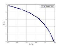 | , | ||
| Test function 4: | ![Test function 4[6].](http://upload.wikimedia.org/wikipedia/commons/thumb/3/3c/Test_function_4_-_Binh.pdf/page1-200px-Test_function_4_-_Binh.pdf.jpg) | |||
| Kursawe function: | 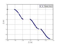 | , . | ||
| Schaffer function N. 1[19] : | 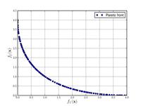 | . Values of from to have been used successfully. Higher values of increase the difficulty of the problem. | ||
| Schaffer function N. 2: |  | . | ||
| Poloni's two objective function: | 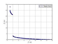 |
| ||
| Zitzler–Deb–Thiele's function N. 1[20] : |  | , . | ||
| Zitzler–Deb–Thiele's function N. 2[20] : | 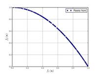 | , . | ||
| Zitzler–Deb–Thiele's function N. 3[20]: | 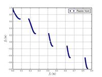 | , . | ||
| Zitzler–Deb–Thiele's function N. 4[20]: | 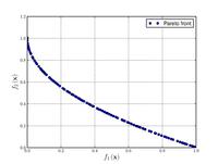 | , , | ||
| Zitzler–Deb–Thiele's function N. 6[20]: |  | , . | ||
| Osyczka and Kundu function[21]: | 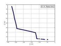 | , , . | ||
| CTP1 function (2 variables)[4],[22]: | ![CTP1 function (2 variables)[4].](http://upload.wikimedia.org/wikipedia/commons/thumb/d/d4/CTP1_function_%282_variables%29.pdf/page1-200px-CTP1_function_%282_variables%29.pdf.jpg) | . | ||
| Constr-Ex problem[4]: | ![Constr-Ex problem[4].](http://upload.wikimedia.org/wikipedia/commons/thumb/6/6f/Constr-Ex_problem.pdf/page1-200px-Constr-Ex_problem.pdf.jpg) | , | ||
| Viennet function: |  | . |


![{\displaystyle {\text{Minimize}}={\begin{cases}f_{1}\left({\boldsymbol {x}}\right)=1-\exp \left[-\sum _{i=1}^{n}\left(x_{i}-{\frac {1}{\sqrt {n}}}\right)^{2}\right]\\f_{2}\left({\boldsymbol {x}}\right)=1-\exp \left[-\sum _{i=1}^{n}\left(x_{i}+{\frac {1}{\sqrt {n}}}\right)^{2}\right]\\\end{cases}}}](https://wikimedia.org/api/rest_v1/media/math/render/svg/3113203c5d455e0e1e6397d57094e80e527b34ba)


![{\displaystyle {\text{Minimize}}={\begin{cases}f_{1}\left({\boldsymbol {x}}\right)=\sum _{i=1}^{2}\left[-10\exp \left(-0.2{\sqrt {x_{i}^{2}+x_{i+1}^{2}}}\right)\right]\\&\\f_{2}\left({\boldsymbol {x}}\right)=\sum _{i=1}^{3}\left[\left|x_{i}\right|^{0.8}+5\sin \left(x_{i}^{3}\right)\right]\\\end{cases}}}](https://wikimedia.org/api/rest_v1/media/math/render/svg/aeb9856144d9869aae4254892ece0fe894dfc152)


![{\displaystyle {\text{Minimize}}={\begin{cases}f_{1}\left(x,y\right)=\left[1+\left(A_{1}-B_{1}\left(x,y\right)\right)^{2}+\left(A_{2}-B_{2}\left(x,y\right)\right)^{2}\right]\\f_{2}\left(x,y\right)=\left(x+3\right)^{2}+\left(y+1\right)^{2}\\\end{cases}}}](https://wikimedia.org/api/rest_v1/media/math/render/svg/9ee5df22af124899c1e268325017ea64e517b51e)


![{\displaystyle {\text{Minimize}}={\begin{cases}f_{1}\left({\boldsymbol {x}}\right)=1-\exp \left(-4x_{1}\right)\sin ^{6}\left(6\pi x_{1}\right)\\f_{2}\left({\boldsymbol {x}}\right)=g\left({\boldsymbol {x}}\right)h\left(f_{1}\left({\boldsymbol {x}}\right),g\left({\boldsymbol {x}}\right)\right)\\g\left({\boldsymbol {x}}\right)=1+9\left[{\frac {\sum _{i=2}^{10}x_{i}}{9}}\right]^{0.25}\\h\left(f_{1}\left({\boldsymbol {x}}\right),g\left({\boldsymbol {x}}\right)\right)=1-\left({\frac {f_{1}\left({\boldsymbol {x}}\right)}{g\left({\boldsymbol {x}}\right)}}\right)^{2}\\\end{cases}}}](https://wikimedia.org/api/rest_v1/media/math/render/svg/f03bdd2b0c7a5af33b0a0fc385f9a9c021635d6e)


Voir aussi
- Fonction d'Ackley
- Fonction de Himmelblau
- Fonction Rastrigin
- Fonction de Rosenbrock
- Fonction shekel
- Fonction binh
Références
- ↑ Thomas Bäck, Evolutionary algorithms in theory and practice : evolution strategies, evolutionary programming, genetic algorithms, Oxford, Oxford University Press, (ISBN 978-0-19-509971-3), p. 328
- ↑ Randy L. Haupt, Sue Ellen Haupt, Practical genetic algorithms with CD-Rom, New York, 2nd, (ISBN 978-0-471-45565-3)
- ↑ Oldenhuis, « Many test functions for global optimizers », Mathworks (consulté le )
- ↑ a b c d et e Deb, Kalyanmoy (2002) Multiobjective optimization using evolutionary algorithms (Repr. ed.). Chichester [u.a.]: Wiley. (ISBN 0-471-87339-X).
- ↑ Binh T. and Korn U. (1997) MOBES: A Multiobjective Evolution Strategy for Constrained Optimization Problems. In: Proceedings of the Third International Conference on Genetic Algorithms. Czech Republic. pp. 176–182
- ↑ a et b Binh T. (1999) A multiobjective evolutionary algorithm. The study cases. Technical report. Institute for Automation and Communication. Barleben, Germany
- ↑ Deb K. (2011) Software for multi-objective NSGA-II code in C. Available at URL: https://www.iitk.ac.in/kangal/codes.shtml
- ↑ Ortiz, « Multi-objective optimization using ES as Evolutionary Algorithm. », Mathworks (consulté le )
- ↑ Whitley, Rana, Dzubera et Mathias, « Evaluating evolutionary algorithms », Artificial Intelligence, Elsevier BV, vol. 85, nos 1-2, , p. 264 (ISSN 0004-3702, DOI 10.1016/0004-3702(95)00124-7)
- ↑ Simionescu, P.A. et Beale, D. « New Concepts in Graphic Visualization of Objective Functions » (September 29 – October 2, 2002) (lire en ligne, consulté le )
—ASME 2002 International Design Engineering Technical Conferences and Computers and Information in Engineering Conference - ↑ « Solve a Constrained Nonlinear Problem - MATLAB & Simulink », www.mathworks.com (consulté le )
- ↑ « Bird Problem (Constrained) | Phoenix Integration » [archive du ] (consulté le )
- ↑ Mishra, « Some new test functions for global optimization and performance of repulsive particle swarm method », MPRA Paper, (lire en ligne)
- ↑ Townsend, « Constrained optimization in Chebfun », chebfun.org, (consulté le )
- ↑ Simionescu, « A collection of bivariate nonlinear optimisation test problems with graphical representations », International Journal of Mathematical Modelling and Numerical Optimisation, vol. 10, no 4, , p. 365–398 (DOI 10.1504/IJMMNO.2020.110704)
- ↑ P.A. Simionescu, Computer Aided Graphing and Simulation Tools for AutoCAD Users, Boca Raton, FL, 1st, (ISBN 978-1-4822-5290-3)
- ↑ Vira Chankong et Yacov Y. Haimes, Multiobjective decision making. Theory and methodology., (ISBN 0-444-00710-5)
- ↑ Fonseca et Fleming, « An Overview of Evolutionary Algorithms in Multiobjective Optimization », Evol Comput, vol. 3, no 1, , p. 1–16 (DOI 10.1162/evco.1995.3.1.1, S2CID 8530790, CiteSeerx 10.1.1.50.7779)
- ↑ J. David Schaffer, Proceedings of the First International Conference on Genetic Algorithms, (OCLC 20004572), « Multiple Objective Optimization with Vector Evaluated Genetic Algorithms »
- ↑ a b c d et e Kalyan Deb, L. Thiele, Marco Laumanns et Eckart Zitzler, Proceedings of the 2002 IEEE Congress on Evolutionary Computation, vol. 1, , 825–830 p. (ISBN 0-7803-7282-4, DOI 10.1109/CEC.2002.1007032, S2CID 61001583), « Scalable multi-objective optimization test problems »
- ↑ Osyczka et Kundu, « A new method to solve generalized multicriteria optimization problems using the simple genetic algorithm », Structural Optimization, vol. 10, no 2, , p. 94–99 (ISSN 1615-1488, DOI 10.1007/BF01743536, S2CID 123433499)
- ↑ Jimenez, Gomez-Skarmeta, Sanchez et Deb, « An evolutionary algorithm for constrained multi-objective optimization », Proceedings of the 2002 Congress on Evolutionary Computation. CEC'02 (Cat. No.02TH8600), vol. 2, , p. 1133–1138 (ISBN 0-7803-7282-4, DOI 10.1109/CEC.2002.1004402, S2CID 56563996)
 Portail des mathématiques


